plotfalsecolours
The plotfalsecolours function creates a false-colour illustration for a given data set.
Usage:
plotfalsecolours(x,y,Y,mode,clabel,climits)
Where:
| Parameter | Description |
x and y | Are the coordinate vectors of the mesh grid. |
Y | Is the data distribution in matrix form. |
mode | Defines the plot mode: ‘lin’ for linear colour scale (default) ‘log’ for logarithmic colour scale |
clabel | Is the colour bar label. |
climits | Specifies the colour bar limits in vector format: [c1 c2] |
Example
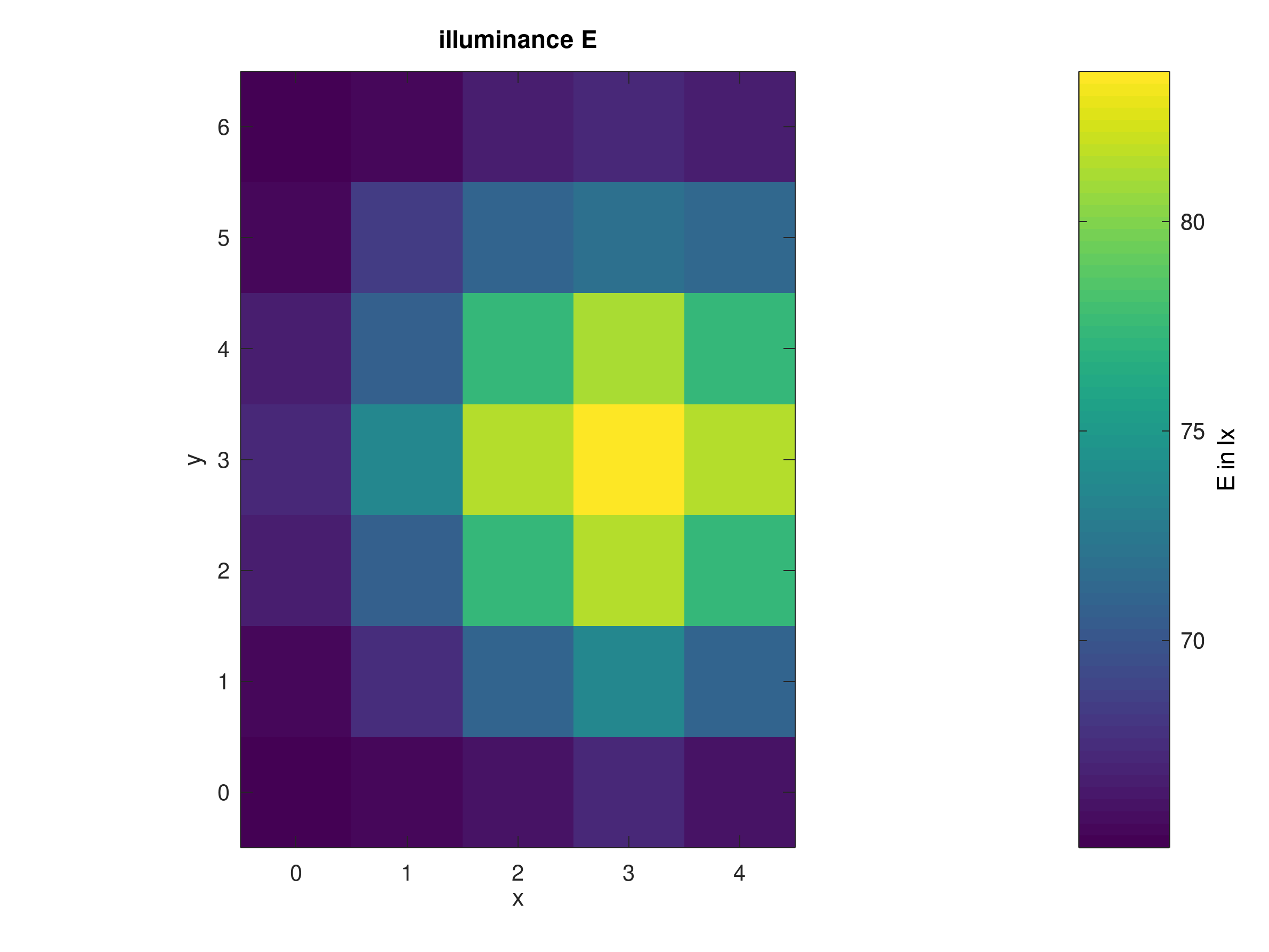
Plot an illuminance distribution on a surface:
x = 0:4;
y = 0:6;
E = [65.0451 65.4281 66.6292 67.1130 66.7063
     65.4280 68.4963 71.0842 71.7268 71.1471
     66.6291 70.7887 77.3848 81.2140 77.3849
     67.1127 73.6917 81.5131 83.5850 81.3887
     66.6291 70.7887 77.3848 81.5566 77.4113
     65.4281 67.4780 70.9568 73.6784 70.8536
     65.0451 65.4280 66.1305 67.1127 66.1305];

plotfalsecolours(x,y,E,'E in lx')
title('illuminance E')
Result:

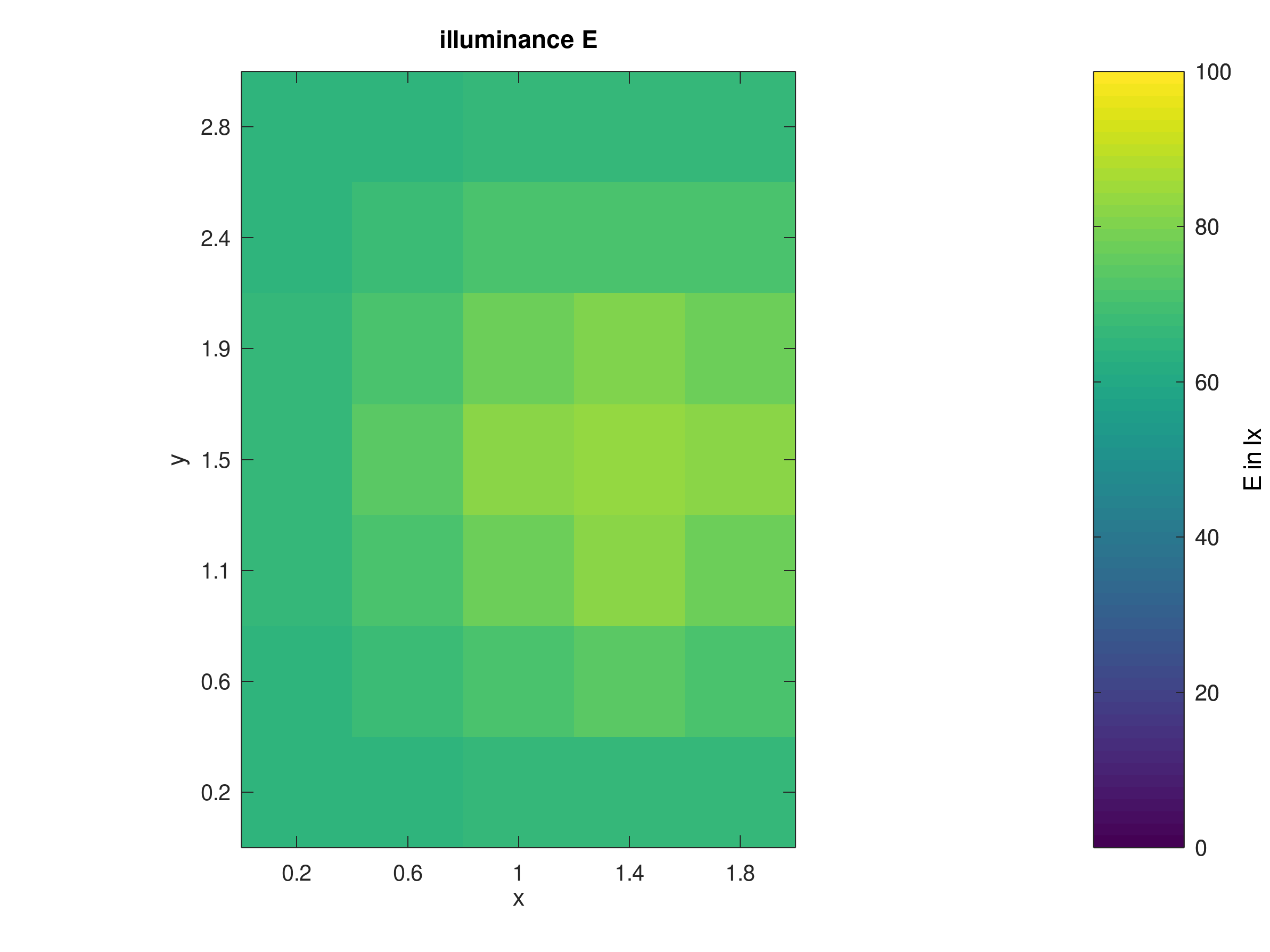
Plot an illuminance distribution of a measurement grid and adjust the colourbar limits from 0 lx to 100 lx:
[x,y] = egrid(2,3);
E = [65.0451 65.4281 66.6292 67.1130 66.7063
     65.4280 68.4963 71.0842 71.7268 71.1471
     66.6291 70.7887 77.3848 81.2140 77.3849
     67.1127 73.6917 81.5131 83.5850 81.3887
     66.6291 70.7887 77.3848 81.5566 77.4113
     65.4281 67.4780 70.9568 73.6784 70.8536
     65.0451 65.4280 66.1305 67.1127 66.1305];

plotfalsecolours(x,y,E,'lin','E in lx',[0 100])
title('illuminance E')
See also: egrid
Result:

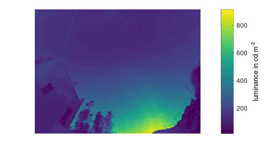
Plot a luminance image:
load('L-image');
plotfalsecolours(L,'luminance in cd m^{-2}')
Result:

Plot a luminance image in log colour scale:
load('L-image');
plotfalsecolours(L,'log','luminance in cd m^{-2}')
Result:

Note for use in Octave: To adjust the colour bar scale limits in'log' mode, use the caxis command with log10 values:
caxis(log10([10 1000]))
Result:
