plotciexy
The plotciexy function plots the CIE 1931 x and y chromaticity diagram.
Note 1:
The plot consists of an background image of 1000 \times 1000 pixels with an inverse y-axis. For additional plotting with the hold command one need to adjust the x and y coordinates accordingly, see also last example:
x = x.*1000;
y = 1000-y.*1000;
Note 2:
In Octave the plotciexy function runs significantly faster using the image package. Consider installing and loading the image package before using the cieplotxy function. It will work without it though.
Install package:
pkg install image
Load package:
pkg load image
By adding the load command to the .octaverc file, octave will load the toolbox automatically at startup.
Note 3:
The plotciexy function just calls another function named cie1931 which contains the actual code to plot the diagram. I have done this in the sake of a better function name but at the same time backwards compability for my own code.
Usage:
plotciexy(x,y,'parameter','value')
Where:
| Parameter | Description |
x and y | Are the to be plotted CIE 1931 x and y chromaticity coordinates. For an empty chromaticity diagram use an emtpy function call: plotciexy, plotciexy() or plotciexy(NaN,NaN) |
'input' | ‘xy’ for CIE 1931 x and y chromaticity coordinates (default) ‘uv’ for CIE 1960 u and v chromaticity coordinates which are transformed to x and y automatically |
'color' | ‘on’ for plotting the diagram filled with the acording colours (default) ‘off’ for plotting the diagram without colours |
'background' | ‘white’ for white background (default) ‘black’ for black background |
'marker' | Marker for the given chromaticity coordinates: ‘+’ (default), ‘o’ , ‘*’ , ‘.’ , ‘x’ , ‘s’ , ‘d’ , ‘^’ , ‘v’ , ‘>’ , ‘<‘ , ‘p’ , ‘h’ , ‘square’ , ‘diamond’ , ‘pentagram’ , ‘hexagram’ |
'markercolor' | Color of the plotted chromaticity markers, default is the standard colour order: 1\times 3 vector or standard colour shortcuts (e.g. ‘b’,’r’,’g’,’c’,’y’,’k’) for uniform [r g b] marker colour n\times 3 [r g b] matrix for n different marker colours |
'markersize' | Size of the plotted chromaticity markers, numeric: default = 1 |
'whitepoints' | Plots additional whitepoints of standard illuminants into the diagram: see: ciewhitepoint For several whitepoints use an cell array: {‘A’,’E’,’D65′,…} |
'planck' | ‘on’ plots the Plancian Locus into the diagram ‘off’ default |
'CCT' | ‘off’ default Plankian Locus must be enabled for the following options: ‘value’ plots an isotemperature line for each given input coordinate ‘range’ plots the lowest and highest isotemperature line for the given coordinates |
'isotemplines' | Plankian Locus must be enabled for the option Plots additional isotemperature lines: [Tcp1 Tcp2 … Tcpn] |
'daylightlocus' | ‘on’ plots the Daylight Locus int the diagram ‘off’ default |
'legendmode' | ‘off’ default ‘on’ shows a legend of the given chromaticity coordinates ‘extended’ shows a legend of the given chromaticity coordinates and corresponding CCT |
'grid' | ‘on’ plots grid lines in the diagram (default) ‘off’ |
'fontsize' | Fontsize of text, numeric, default = 8 |
'zoom' | Zooms into a certain region of the diagram, numeric vector [x1 x2 y1 y2] default = [0 0.8 0 0.9] |
Examples
Plot CIE 1931 x and y chromaticity diagram:
plotciexy
Result:

Plot data in CIE 1931 x and y chromaticity diagram:
x = 0.3456;
y = 0.2456;
plotciexy(x,y)
Result:

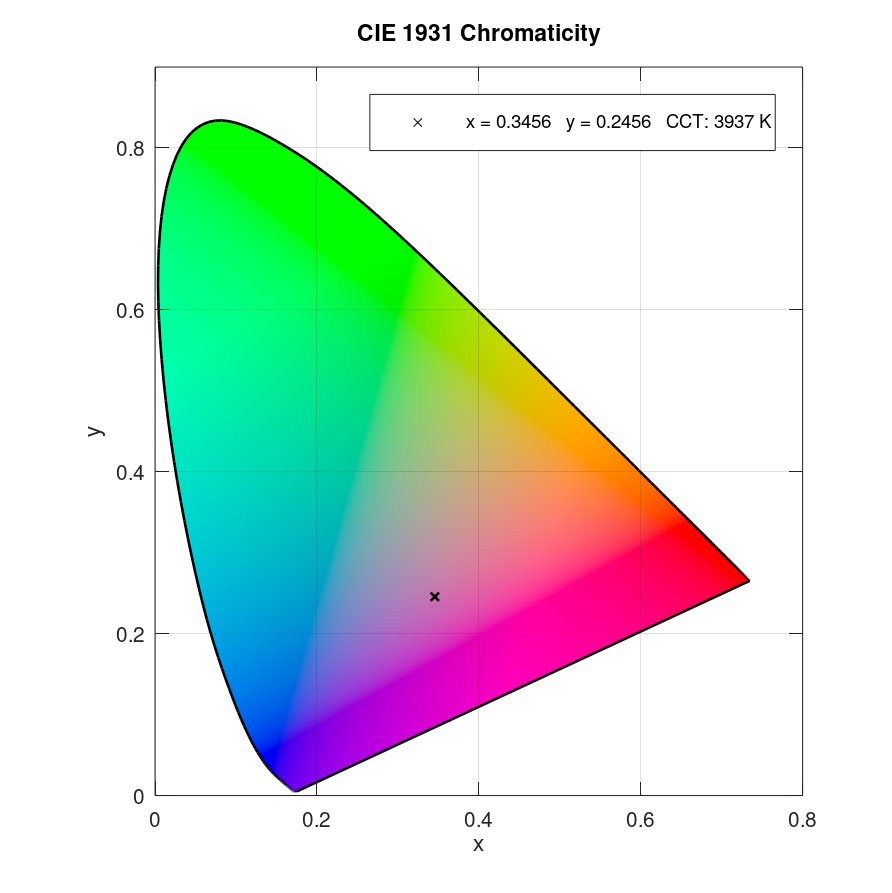
Plot data in CIE 1931 x and y chromaticity diagram with specified marker with extended legend:
x = 0.3456;
y = 0.2456;
plotciexy(x,y,'marker','x','markercolor','k',...
'markersize',4,'legendmode','extended')
Result:
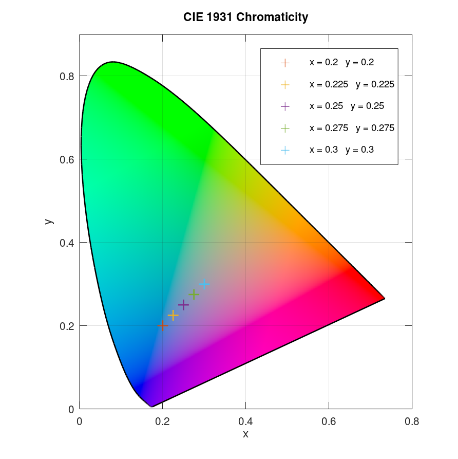
Plot several data points in CIE 1931 x and y chromaticity diagram with legend:
x = linspace(0.2,0.3,5);
y = linspace(0.2,0.3,5);
plotciexy(x,y,'legendmode','on')
Result:
Plot several data points in CIE 1931 x and y chromaticity diagram with different marker and colours:
x = linspace(0.2,0.3,5);
y = linspace(0.2,0.3,5);
c = colours(5);
plotciexy(x,y,'marker','.','markercolor',c,...
'markersize',8,'legendmode','on')
See also: colours
Result:

Plot several data points in CIE 1931 x and y chromaticity diagram with planckian locus and CCT range:
x = linspace(0.3,0.4,5);
y = linspace(0.3,0.4,5);
plotciexy(x,y,'markercolor',[1 0 0],'planck','on','CCT','range')
Result:

Plot several data points in CIE 1931 x and y chromaticity diagram with planckian locus and isotemperature lines:
x = linspace(0.3,0.4,5);
y = linspace(0.3,0.375,5);
plotciexy(x,y,'marker','.','markercolor',[1 0 0],...
'planck','on','CCT','value')
Result:

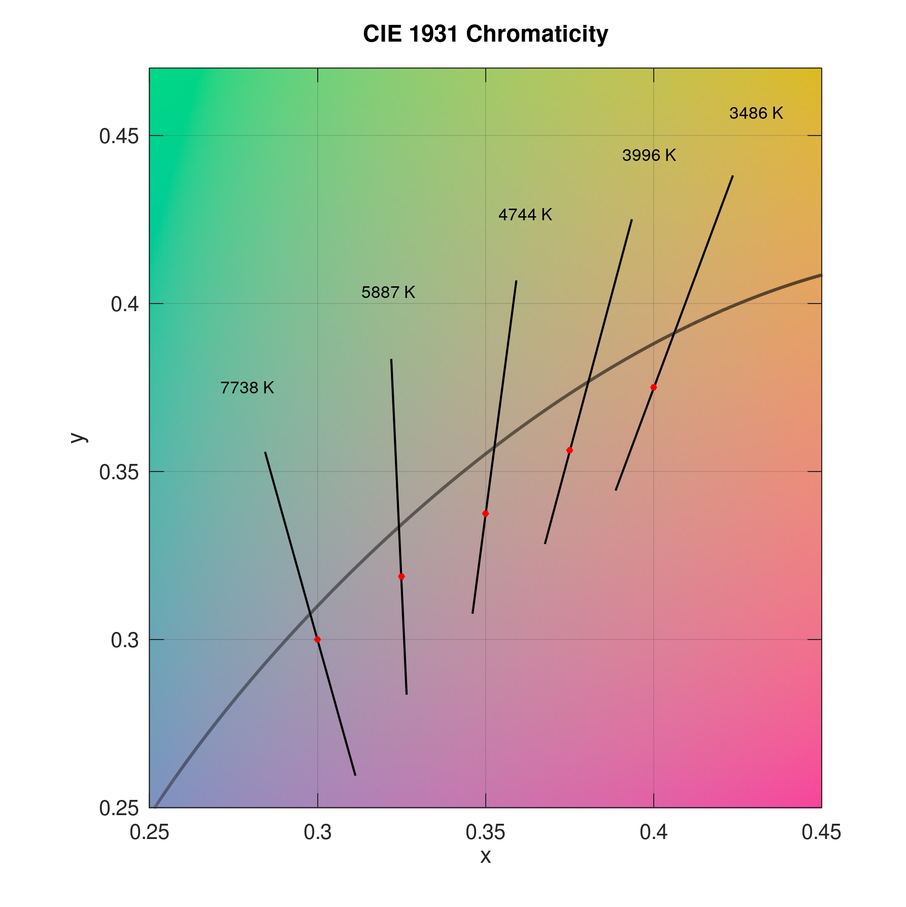
Plot several data points in CIE 1931 x and y chromaticity diagram with planckian locus and isotemperature lines and zoom to certain region:
x = linspace(0.3,0.4,5);
y = linspace(0.3,0.375,5);
plotciexy(x,y,'marker','.','markercolor',...
[1 0 0],'planck','on','CCT','value','zoom',[0.25 0.45 0.25 0.47])
Result:
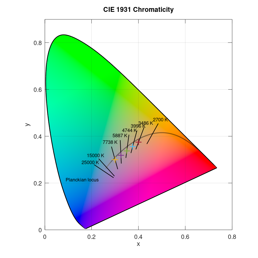
Plot several data points in CIE 1931 x and y chromaticity diagram with planckian locus and additional isotemperature lines:
x = linspace(0.3,0.4,5);
y = linspace(0.3,0.375,5);
iso = [2700 15000 25000];
plotciexy(x,y,'planck','on','CCT','value','isotemplines',iso)
Result:
Plot data in CIE 1931 x and y chromaticity diagram using u and v input:
u = 0.2630;
v = 0.2004;
plotciexy(u,v,'input','uv')
Result:

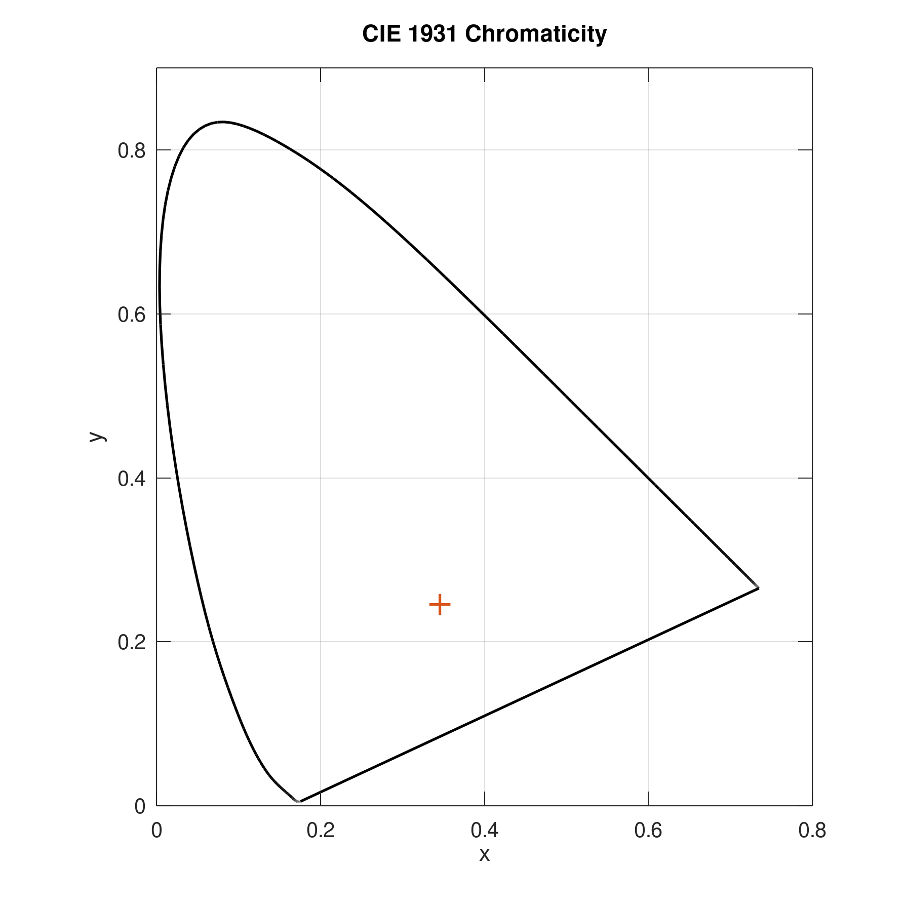
Plot data in CIE 1931 x and y chromaticity diagram without colour:
x = 0.3456;
y = 0.2456;
plotciexy(x,y,'Color','off')
Result:
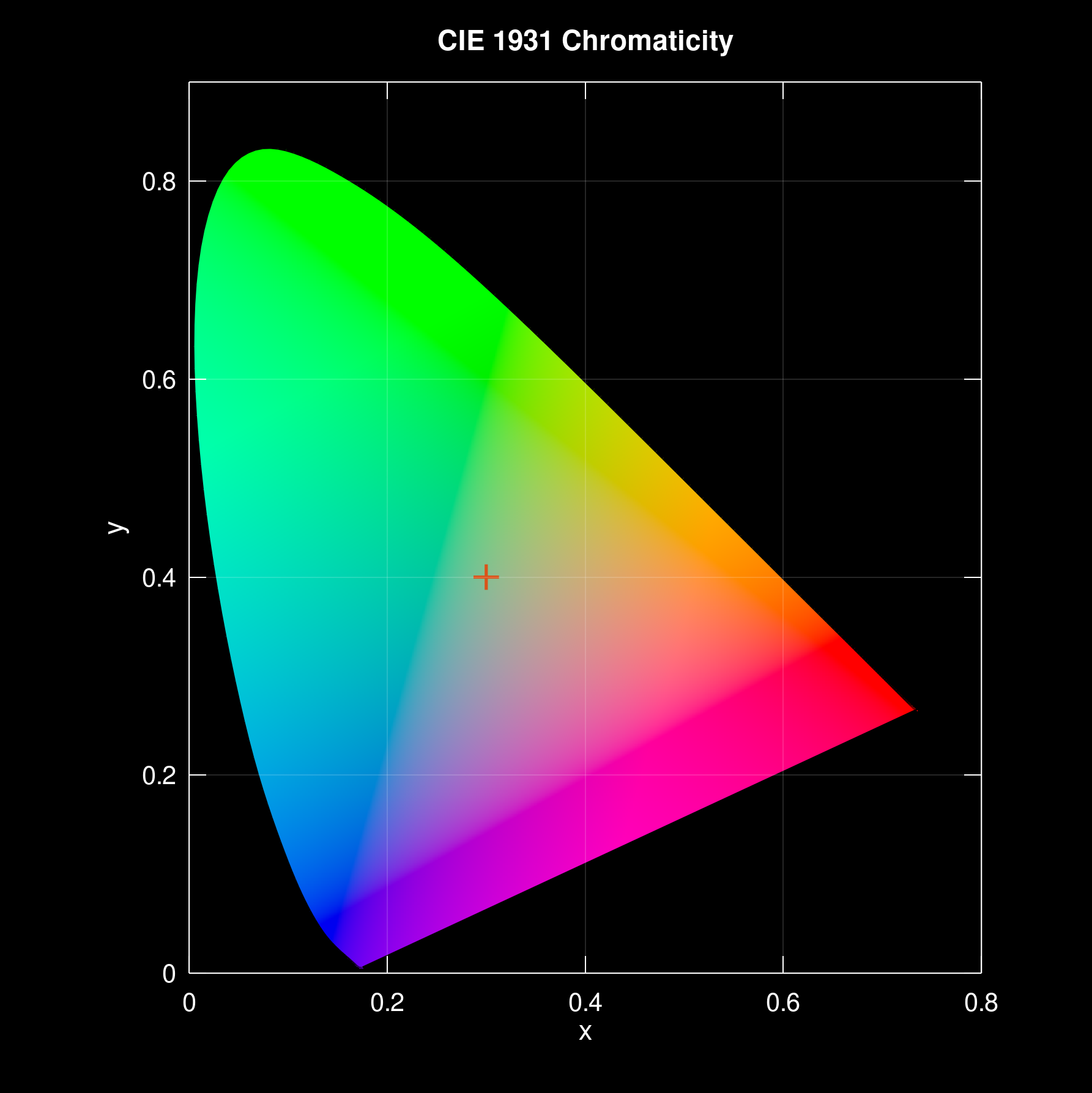
Plot data in CIE 1931 x and y chromaticity diagram on black background:
plotciexy(0.3,0.4,'Background','black')
Result:
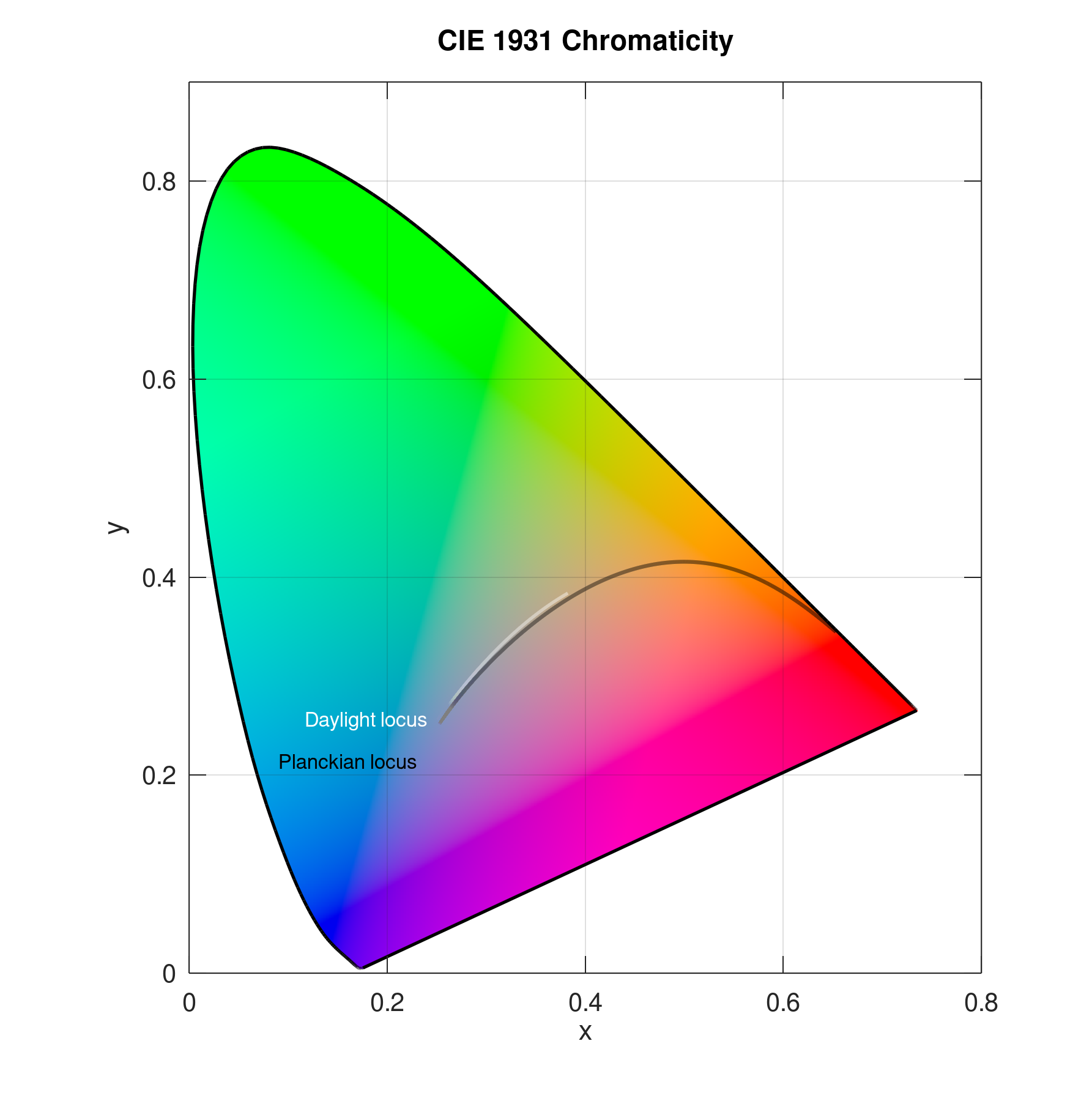
Plot CIE 1931 x and y chromaticity diagram with with no data points but Planckian and daylight locus:
plotciexy(NaN,NaN,'Planck','on','DaylightLocus','on')
Result:
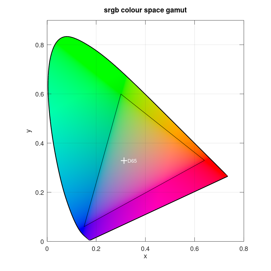
Plot CIE 1931 x and y chromaticity diagram with whitepoint ‘D65’ and add srgb colour space gamut:
plotciexy(NaN,NaN,'whitepoints','D65')
hold on
% srgb colour space gamut according to https://en.wikipedia.org/wiki/SRGB
x = [0.64 0.30 0.15 0.64];
y = [0.33 0.60 0.06 0.33];
% transform data for plot on image
x = x.*1000;
y = 1000-y.*1000;
% plot srgb colour space gamut
plot(x,y,'k')
title('srgb colour space gamut')
hold off
Result:
References
ISO/CIE 12664-3:2019(E): Colorimetry – Part 3: CIE tristimulus values. Commission International de l’Éclairage (CIE), Vienna Austria, 2019. URL: https://cie.co.at/publications/colorimetry-part-3-cie-tristimulus-values-2
CIE 15:2018: Colorimetry, 4th Edition. Commission Internationale de l’Eclairage (CIE), Vienna Austria, 2018, ISBN: 978-3-902842-13-8 , DOI: 10.25039/TR.015.2018. URL: https://cie.co.at/publications/colorimetry-4th-edition
>> x = 0.3456;
>> y = 0.2456;
>> plotciexy(x,y)
Undefined function or variable ‘polyshape’.
Error in cie1931 (line 305)
poly = polyshape({[1 1000 1000 1 1],ciex.*1000},{[1 1 1000 1000 1],(1-ciey).*1000});
Error in plotciexy (line 81)
cie1931(x,y)
The polyshape function is a basic Matlab function introduced with version 2017b. I assume you are using an older version, which lacks this function.
Since the function is not strictly needed to plot the chromaticity diagram, I removed the polyshape function from the plotciexy,uv,uv_ toolbox functions, the new version 1.12 is now available on github.
But I would recommend using an up-to-date Matlab version or – if that is not possible – the alternative GNU Octave, since you might also encounter other problems with the toolbox.